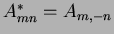
The Zernike polynomials were first proposed in 1934 by Zernike [22]. Their moment formulation appears to be one of the most popular, outperforming the alternatives [19] (in terms of noise resilience, information redundancy and reconstruction capability). The pseudo-Zernike formulation proposed by Bhatia and Wolf [3] further improved these characteristics. However, here we study the original formulation of these orthogonal invariant moments.
Complex Zernike moments [18] are constructed using a set of complex polynomials which form a complete orthogonal basis set defined on the unit disc 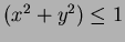 . They are expressed as
 Two dimensional Zernike moment:
![\begin{displaymath}
A_{mn} = \frac{m+1}{\pi} \int_{x} \int_{y} f(x,y)[V_{mn}(x,y)]^{*} ~dx~dy~~~~~\mbox{where $x^{2} + y^{2} \leq ~1$}
\end{displaymath}](http://homepages.inf.ed.ac.uk/rbf/CVonline/LOCAL_COPIES/SHUTLER3/img171.png) | (49) |
 and defines the order,
  is the function being described and
  denotes the complex conjugate. While
  is an integer (that can be positive or negative) depicting the angular dependence, or rotation, subject to the conditions:
 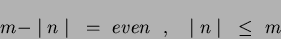 | (50) |
 is true. The Zernike polynomials [22]
  Zernike polynomial expressed in polar coordinates are:
 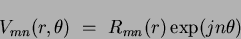 | (51) |
 are defined over the unit disc,
  and
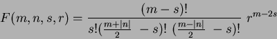
and  is the orthogonal radial polynomial, defined asOrthogonal radial polynomial:
 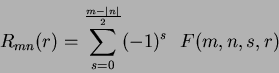 | (52) |
 | (53) |
 and it must be noted that if the conditions in Equation 1.50 are not met, then
  . The first six orthogonal radial polynomials are: Figure 1.6 shows eight such radial responses, where it can been seen that the polynomials become more grouped, as they approach the edge of the unit disc (
 approaches unity). (Care must be taken with regard to the accuracy of these polynomial calculations as the factorial operations can quickly produce large integer values, even at relatively low order
  ). The difference between these orthogonal polynomials and the non-orthogonal monomials can be seen by comparing Figure 1.6 with Figure 1.2.
Figure 1.6: Eight orthogonal radial polynomials plotted for increasing .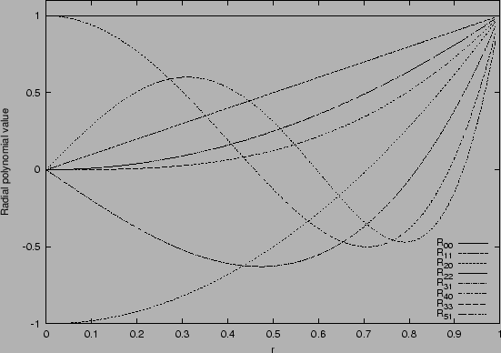 |
 is the current pixel then Equation 1.49 becomes:
 ![\begin{displaymath}
A_{mn} = \frac{m+1}{\pi} \sum_{x} \sum_{y} P_{xy}[V_{mn}(x,y)]^{*} ~~~~~\mbox{where $x^{2} + y^{2} \leq ~1$}
\end{displaymath}](http://homepages.inf.ed.ac.uk/rbf/CVonline/LOCAL_COPIES/SHUTLER3/img195.png) | (55) |
 axis to the vector Polar co-ordinate radius,
  Polar co-ordinate angle, by convention measured from the positive axis in a counter clockwise direction. The mapping from Cartesian to polar coordinates is:
 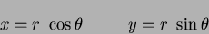 | (56) |
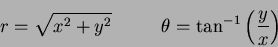 | (57) |
 in practice is often defined over the interval
 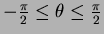 , so care must be taken as to which quadrant the Cartesian coordinates appear in. Translation and scale invariance can be achieved by normalising the image using the Cartesian moments prior to calculation of the Zernike moments [7]. Translation invariance is achieved by moving the origin to the image's COM, causing
 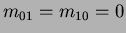 . Following this, scale invariance is produced by altering each object so that its area (or pixel count for a binary image) is
  , where
  is a predetermined value. Both invariance properties (for a binary image) can be achieved using :
 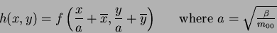 | (58) |
 is the new translated and scaled function. The error involved in the discrete implementation can be reduced by interpolation. If the coordinate calculated by Equation 1.58 does not coincide with an actual grid location, the pixel value associated with it is interpolated from the four surrounding pixels. As a result of the normalisation, the Zernike moments
  and
and  are set to known values. is set to zero, due to the translation of the shape to the centre of the coordinate system. This however will be affected by a discrete implementation where the error in the mapping will decrease as the shape (being mapped) size (or pixel-resolution) increases. is dependent on
  , and thus on :
  | (59) |
 is the angle of rotation,
  is the Zernike moment of the rotated image and
  is the Zernike moment of the original image then:
 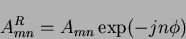 | (60) |
Subsections


 Next: A note on image Up: Orthogonal moments Previous: Legendre momentsJamie Shutler 2002-08-15