최근에 Learning from demonstration with model-based Gaussian process, CORL, 2019 (Learning from demonstration with model-based Gaussian process) 를 읽다가 GMR에 급 관심이 생겨서 맷랩으로 한번 구현을 해봤다. Input과 output의 joint distribution을 GMM으로 모델링하고, prediction은 conditional Gaussian을 이용해서 하는 재밌는 방법이다.
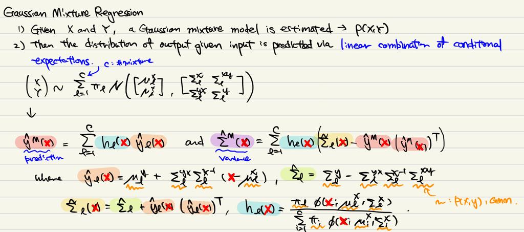
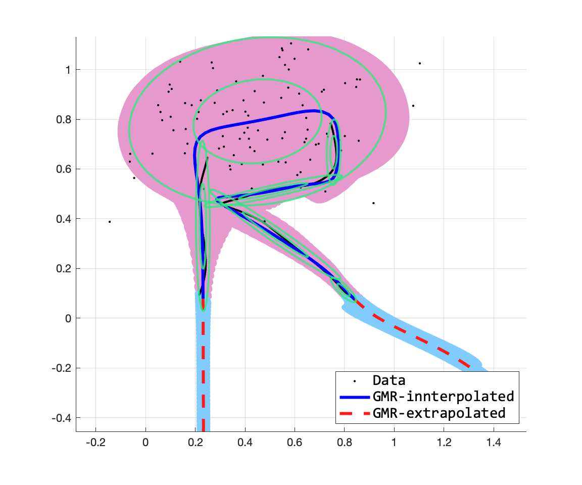
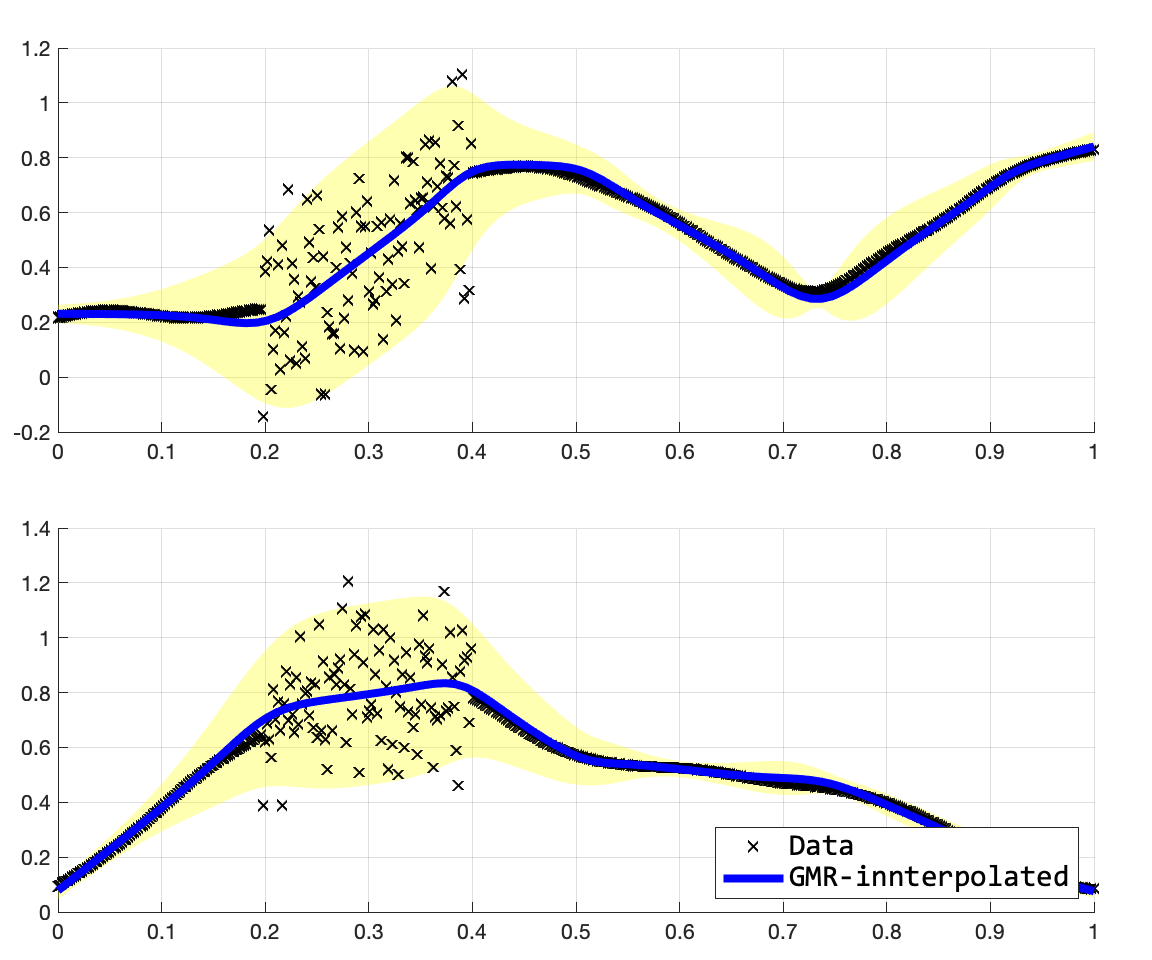
위의 수식이 GMR의 수식이다. 내가 참고한 논문에서는 $\hat{\Sigma}$를 적을 때, 괄호가 빠져있어서 조금 어려움이 있었는데, 모 논문들이 다 그렇지모. 여튼 위의 수식을 구현해보면 아래의 그림을 얻을 수 있다. 여기서 주의깊게 보고 싶었던 것은 이차원의 출력들 사이의 dependency가 어떻게 잡히나, 그리고 이를 통해서 extrapoloation이 얼마나 잘 되는지였는데, 나쁘지 않다.
알고리즘은 대략적으로 아래와 같이 굴러간다.
1. Input과 output을 한번에 GMM으로 모델링을 한다.
2. X, Y, XY 파트에 대해서 mu와 var를 구한다.
3. Prediction을 할 때는 conditional Gaussian distribution의 mu, var를 쓴다.
여기서 중요한 부분은 step1의 GMM을 구하는 것인데, 데이터가 몇 개이든 상관이 없이, k개의 가우시안 분포의 mu, var를 쓸 수 밖에 없게된다. 이는 데이터의 사소한 디테일을 뭉개버리는 효과가 생긴다. 그래서 노이지한 경우에 좋은 결과가 나오 수 있으나, 사소한 디테일이 중요한 문제에는 적합하지 않다는 생각이 든다.
여기에 추가로 든 생각은 모든 것이 linear하기 떄문에 생기는 한계가 분명하다.
코드
1. main.m
% Configuration
RECOLLECT = false;
mat_name = 'gmrgp_data.mat';
if exist(mat_name,'file') && (~RECOLLECT)
l = load(mat_name);
xs = l.xs;
else
% Get 2D trajectories using mouse clicks
fig = figure(1); hold on;
rectangle('Position',[0 0 1 1],'Curvature',0.1)
axis equal; axis([0,1,0,1]); grid on;
title('Press [q] to stop.','FontSize',15,'FontName','Consolas');
xs = [];
while true
% Get click position
[x1,x2,BUTTON] = ginput(1);
switch BUTTON
case 1 % clicked
xs = [xs; x1,x2]; % append
plot(x1,x2,'bo');
drawnow;
case 113 % q
break
otherwise
end
end
% Save
save(mat_name,'xs');
fprintf(2,'[%s] saved.\n',mat_name);
end
n = size(xs,1); % #data
fprintf('[%d] number of data collected.\n',n);
% Get GRP and interpolate the points
ts = linspace(0,1,n)';
hyp = [1,1,0.01];
sig2w = 1e-6;
n_test = 500; % number of data for gmr
t_test = linspace(0,1,n_test)';
lgrp = get_grp(ts,xs,t_test,ones(n,1),ones(n_test,1),...
'kernel_levrq',hyp,sig2w,hyp,sig2w);
sampled_paths = sample_grp(lgrp,20); % sample
% plot_grp(lgrp,'n_sample',0);
X = t_test;
Y = lgrp.mu;
d_x = size(X,2); d_y = size(Y,2);
fprintf('[%d] number of training data for GMR.\n',size(X,1));
% Add some noise to Y
idx_fr = round(n_test*0.2);
idx_to = round(n_test*0.4);
Y(idx_fr:idx_to,:) = Y(idx_fr:idx_to,:) + 0.2*randn(size(Y(idx_fr:idx_to,:)));
% Plot points and trajectory
PLOT_INTERPOLATED = 0;
if PLOT_INTERPOLATED
figure(); hold on;
rectangle('Position',[0 0 1 1],'Curvature',0.1)
axis equal; axis([0,1,0,1]); grid on;
for i_idx = 1:length(sampled_paths)
sampled_path = sampled_paths{i_idx};
% plot(sampled_path(:,1),sampled_path(:,2),'k-','LineWidth',1);
end
plot(xs(:,1),xs(:,2),'bo','MarkerSize',20,'LineWidth',3); % training points
plot(Y(:,1),Y(:,2),'b-','LineWidth',3); % interpoloated trajectory
end
% Train GMM
addpath('EmGm')
k = 10; % #mixtures
n_reset = 10;
z_list = cell(1,n_reset); model_list = cell(1,n_reset); liks = zeros(1,n_reset);
for r_idx = 1:n_reset
rng(r_idx);
[z,model,llh] = mixGaussEm([X,Y]',k,'VERBOSE',0); % train
z_list{r_idx} = z; model_list{r_idx} = model;
liks(r_idx) = llh(end);
end
[~,max_idx] = max(liks);
z = z_list{max_idx}; model = model_list{max_idx};
k = length(unique(z));
d = size(model.mu,1);
gmm.k = k;
eps_gmr_x = 1e-6;
eps_gmr_y = 1e-4;
for k_idx = 1:k
gmm.pi{k_idx} = model.w(k_idx);
gmm.mu_x{k_idx} = model.mu(1,k_idx);
gmm.mu_y{k_idx} = model.mu(2:3,k_idx);
gmm.sig_x{k_idx} = model.Sigma(1,1,k_idx) + eps_gmr_x*eye(d_x,d_x);
gmm.sig_y{k_idx} = model.Sigma(2:3,2:3,k_idx) + eps_gmr_y*eye(d_y,d_y);
gmm.sig_xy{k_idx} = model.Sigma(1,2:3,k_idx);
gmm.sig_yx{k_idx} = model.Sigma(2:3,1,k_idx);
end
% Plot with output GMM information
PLOT_GMM_Y = false;
if PLOT_GMM_Y
figure(); hold on;
rectangle('Position',[0 0 1 1],'Curvature',0.1)
colors = hsv(k);
for k_idx = 1:k
elpt = ellipsedata(gmm.sig_y{k_idx},gmm.mu_y{k_idx},100,[1]);
plot(elpt(:,1:2:end),elpt(:,2:2:end),'-','Color',colors(k_idx,:),'LineWidth',2);
end
plot(xs(:,1),xs(:,2),'ko','MarkerSize',20,'LineWidth',3); % training points
plot(Y(:,1),Y(:,2),'k-','LineWidth',3); % interpoloated trajectory
axis equal; axis([0,1,0,1]); grid on;
end
% First, run Gaussian mixture regression
n_interp = 100;
x_interp = linspace(0.0,1.0,n_interp);
y_gmr_interp = zeros(n_interp,2);
sig_gmr_interp = cell(n_interp,1);
for i_idx = 1:n_interp
gmr = get_gmr(x_interp(i_idx),gmm);
y_gmr_interp(i_idx,:) = gmr.yhat_M';
sig_gmr_interp{i_idx} = gmr.sighat_M;
end
% Extrapolate on both directions
extrap_rate = 0.2;
n_extrap = round(n_interp*extrap_rate*2);
x_extrap1 = linspace(-extrap_rate,0.0,n_extrap);
y_gmr_extrap1 = zeros(n_extrap,2);
sig_gmr_extrap1 = cell(n_extrap,1);
for i_idx = 1:n_extrap
gmr = get_gmr(x_extrap1(i_idx),gmm);
y_gmr_extrap1(i_idx,:) = gmr.yhat_M';
sig_gmr_extrap1{i_idx} = gmr.sighat_M;
end
x_extrap2 = linspace(1.0,1.0+extrap_rate,n_extrap);
y_gmr_extrap2 = zeros(n_extrap,2);
sig_gmr_extrap2 = cell(n_extrap,1);
for i_idx = 1:n_extrap
gmr = get_gmr(x_extrap2(i_idx),gmm);
y_gmr_extrap2(i_idx,:) = gmr.yhat_M';
sig_gmr_extrap2{i_idx} = gmr.sighat_M;
end
% Plot GMR results
fig = figure(); set_fig_size(fig,[0.1,0.5,0.3,0.4]);
hold on;
colors = hsv(k);
PLOT_GMR_ELPT = true;
if PLOT_GMR_ELPT
for i_idx = 1:1:n_interp
y = y_gmr_interp(i_idx,:);
sig = sig_gmr_interp{i_idx};
elpt = ellipsedata(sig,y,100,[2]);
% plot(elpt(:,1:2:end),elpt(:,2:2:end),'-','Color','k','LineWidth',1);
patch(elpt(:,1:2:end),elpt(:,2:2:end),0,'FaceColor',[0.9,0.6,0.8],...
'EdgeColor','none','FaceAlpha',1.0);
end
for i_idx = 1:1:n_extrap
y = y_gmr_extrap1(i_idx,:);
sig = sig_gmr_extrap1{i_idx};
elpt1 = ellipsedata(sig,y,100,[2]);
% plot(elpt1(:,1:2:end),elpt1(:,2:2:end),'--','Color','k','LineWidth',1);
patch(elpt1(:,1:2:end),elpt1(:,2:2:end),0,'FaceColor',[0.5,0.8,1],...
'EdgeColor','none','FaceAlpha',1.0);
y = y_gmr_extrap2(i_idx,:);
sig = sig_gmr_extrap2{i_idx};
elpt2 = ellipsedata(sig,y,100,[2]);
% plot(elpt2(:,1:2:end),elpt2(:,2:2:end),'--','Color','k','LineWidth',1);
patch(elpt2(:,1:2:end),elpt2(:,2:2:end),0,'FaceColor',[0.5,0.8,1],...
'EdgeColor','none','FaceAlpha',1.0);
end
end
% rectangle('Position',[0 0 1 1],'Curvature',0.1,'LineWidth',3)
% plot(xs(:,1),xs(:,2),'ko','MarkerSize',13,'LineWidth',2); % training points
hdata = plot(Y(:,1),Y(:,2),'k.','LineWidth',1); % GMR output training data
hin = plot(y_gmr_interp(:,1),y_gmr_interp(:,2),'-',...
'Color',[0.0,0.0,1.0],'LineWidth',3); % interpoloated trajectory
hex = plot(y_gmr_extrap1(:,1),y_gmr_extrap1(:,2),'--',...
'Color',[1.0,0.1,0.1],'LineWidth',3); % extrapolated trajectory
plot(y_gmr_extrap2(:,1),y_gmr_extrap2(:,2),'--',...
'Color',[1.0,0.1,0.1],'LineWidth',3); % extrapolated trajectory
PLOT_GMM = true;
if PLOT_GMM
for k_idx = 1:k
elpt = ellipsedata(gmm.sig_y{k_idx},gmm.mu_y{k_idx},100,[1,2]);
% col = colors(k_idx,:);
col = [0.2,0.9,0.5,0.8];
plot(elpt(:,1:2:end),elpt(:,2:2:end),'-','Color',col,'LineWidth',2);
end
end
legend([hdata,hin,hex],{'Data','GMR-innterpolated','GMR-extrapolated'},...
'FontSize',15,'FontName','Consolas','Location','SouthEast');
axis equal; grid on;
set(gcf,'Color','w');
% Plot each dim separately
sig_vec = zeros(n_interp,2);
for i_idx = 1:n_interp
sig = sig_gmr_interp{i_idx};
sig_vec(i_idx,:) = sqrt([sig(1,1),sig(2,2)]);
end
fig = figure(); set_fig_size(fig,[0.1,0.1,0.3,0.4]);
xm = 0.1; ym = 0.1;
subaxes(fig,2,1,1,xm,ym); hold on; grid on;
h_fill = fill([x_interp';flipud(x_interp')],...
[y_gmr_interp(:,1)-2*sig_vec(:,1);flipud(y_gmr_interp(:,1)+2*sig_vec(:,1))],...
'y','LineStyle','none'); % grp 2std
set(h_fill,'FaceAlpha',0.3);
plot(X,Y(:,1),'kx');
plot(x_interp',y_gmr_interp(:,1),'b-','LineWidth',4);
subaxes(fig,2,1,2,xm,ym); hold on; grid on;
h_fill = fill([x_interp';flipud(x_interp')],...
[y_gmr_interp(:,2)-2*sig_vec(:,2);flipud(y_gmr_interp(:,2)+2*sig_vec(:,2))],...
'y','LineStyle','none'); % grp 2std
set(h_fill,'FaceAlpha',0.3);
hd = plot(X,Y(:,2),'kx');
hgmr = plot(x_interp',y_gmr_interp(:,2),'b-','LineWidth',4);
legend([hd,hgmr],{'Data','GMR-innterpolated'},...
'FontSize',15,'FontName','Consolas','Location','SouthEast');
set(gcf,'Color','w');
2. get_gmr.m
function gmr = get_gmr(x_in,gmm)
% First compute h_l, yhat_l, sighat_l, sigtilde_l
yhat_k = cell(1,gmm.k);
sighat_k = cell(1,gmm.k);
h_k = cell(1,gmm.k);
sigtilde_k = cell(1,gmm.k);
eps_h_x = 1e-2; % some eps for computing h_k(x) <= hyper-parameter
h_den = 0;
for k_idx = 1:gmm.k
h_den = h_den + gmm.pi{k_idx}*normpdf(x_in,gmm.mu_x{k_idx},eps_h_x+sqrt(gmm.sig_x{k_idx}));
end
for k_idx = 1:gmm.k
yhat_k{k_idx} = gmm.mu_y{k_idx} + gmm.sig_yx{k_idx}/gmm.sig_x{k_idx}*(x_in-gmm.mu_x{k_idx});
sighat_k{k_idx} = gmm.sig_y{k_idx} - gmm.sig_yx{k_idx}/gmm.sig_x{k_idx}*gmm.sig_xy{k_idx};
sigtilde_k{k_idx} = sighat_k{k_idx} + yhat_k{k_idx}*yhat_k{k_idx}';
h_k{k_idx} = gmm.pi{k_idx}*normpdf(x_in,gmm.mu_x{k_idx},eps_h_x+sqrt(gmm.sig_x{k_idx}))/h_den;
end
% Predice output
yhat_M = 0;
for k_idx = 1:gmm.k
yhat_M = yhat_M + h_k{k_idx}*yhat_k{k_idx};
end
sighat_M = 0;
for k_idx = 1:gmm.k
sighat_M = sighat_M + (h_k{k_idx}*(sigtilde_k{k_idx}-yhat_M*yhat_M'));
end
% Append
gmr.yhat_k = yhat_k;
gmr.sighat_k = sighat_k;
gmr.h_k = h_k;
gmr.sigtilde_k = sigtilde_k;
gmr.yhat_M = yhat_M;
gmr.sighat_M = sighat_M;
3. get_grp.m
function grp = get_grp(t_anchor,x_anchor,t_test,l_anchor,l_test,...
kfun_str,hyp_mu,sig2w_mu,hyp_var,sig2w_var)
%
% Get Gaussian Random Path
%
t_anchor = reshape(t_anchor,[],1);
t_test = reshape(t_test,[],1);
n_anchor = size(t_anchor,1);
n_test = size(t_test,1);
xdim = size(x_anchor,2);
kfun = str2func(kfun_str);
% Make GRP mean zero
x_anchor_mu = mean(x_anchor);
x_anchor_mz = x_anchor - x_anchor_mu;
% Define GRP-mu kernel matrices
% l_anchor_mu = ones(size(l_anchor));
l_anchor_mu = l_anchor;
% l_test_mu = ones(size(l_test));
l_test_mu = l_test;
K_ta_mu = kfun(t_test,t_anchor,l_test_mu,l_anchor_mu,hyp_mu);
K_aa_mu = kfun(t_anchor,t_anchor,l_anchor_mu,l_anchor_mu,hyp_mu) ...
+ sig2w_mu*eye(n_anchor,n_anchor);
grp_mu = K_ta_mu/K_aa_mu*x_anchor_mz + x_anchor_mu;
% Define GRP-var kernel matrices
l_test_var = l_test;
K_ta_var = kfun(t_test,t_anchor,l_test_var,l_anchor,hyp_var);
K_aa_var = kfun(t_anchor,t_anchor,l_anchor,l_anchor,hyp_var) ...
+ sig2w_var*eye(n_anchor,n_anchor);
K_tt_var = kfun(t_test,t_test,l_test_var,l_test_var,hyp_var) + 1e-8*eye(n_test,n_test);
grp_var_mtx = K_tt_var - K_ta_var/K_aa_var*K_ta_var' + 1e-8*max(K_tt_var(:))*eye(n_test,n_test);
grp_var_mtx = 0.5*(grp_var_mtx+grp_var_mtx')/2;
grp_var = diag(grp_var_mtx);
grp_std = sqrt(max(0,grp_var));
% Save grp struct
grp = struct('mu',grp_mu,'var',grp_var,'std',grp_std,...
't_anchor',t_anchor,'x_anchor',x_anchor,'t_test',t_test,...
'l_anchor',l_anchor,'l_test',l_test,...
'n_anchor',n_anchor,'n_test',n_test,...
'xdim',xdim,...
'K_aa_mu',K_aa_mu,'K_ta_mu',K_ta_mu,...
'K',grp_var_mtx,'x_anchor_mu',x_anchor_mu,...
'kfun_str',kfun_str,'kfun',kfun,...
'hyp_mu',hyp_mu,'sig2w_mu',sig2w_mu,...
'hyp_var',hyp_var,'sig2w_var',sig2w_var);
4. kernel_levrq.m
function K = kernel_levrq(X1, X2, L1, L2, hyp)
%
% Rational Quadratic Kernel
%
n1 = size(X1, 1);
n2 = size(X2, 1);
d1 = size(X1, 2);
d2 = size(X2, 2);
if d1 ~= d2, fprintf(2, 'Data dimension missmatch! \n'); end
% Kernel hyperparameters
beta = hyp(1); % gain
gamma = hyp(2:end-1); % length parameters (the bigger, the smoother)
alpha = hyp(end); % RQ alpha (the bigger, the smoother)
% Make each leverave vector a column vector
L1 = reshape(L1,[],1);
L2 = reshape(L2,[],1);
% Compute the leveraged kernel matrix
x_dists = pdist2(X1./gamma, X2./gamma, 'euclidean').^2;
l_dists = pdist2(L1, L2, 'cityblock');
K = beta*(1+1/2/alpha*x_dists).^(-alpha) ...
.*cos(pi/2*l_dists) ;
% Limit condition number
if n1 == n2 && n1 > 1 && 0
sig = 1E-10;
K = K + sig*eye(size(K));
end
5. ellipsedata.m
function elpt = ellipsedata(covmat,center,numpoints,sigmarule,varargin)
%% Ellipsedata V1.001
%
% Construct data points of ellipses representing contour curves of Gaussian
% distributions with any covariance and mean value.
%
%% Example
%
% In this example, the funcion ellipsedata constructs three ellipses of 100
% points each representing the contour curves corresponding to standard deviations
% of 1, 2 and 3 for a Gaussian distribution with covariance matrix given by
% [4,1;1,1] and mean value given by [3,3].
%
% elpt=ellipsedata([4,1;1,1],[3,3],100,[1,2,3]);
%
% The results can be plot as follows
%
% plot(elpt(:,1:2:end),elpt(:,2:2:end));
%
%% Input arguments
%
% covmat:
% Covariance matrix of a bivariate Gaussian distribution. Must be of
% size 2x2, symmetric and positive definite. If the format is not
% correct, an error is triggered. If the matrix is not symmetric, it
% is symmetrized by adding its transpose and dividing by 2.
%
% center:
% The center (mean value) of the bivariate Gaussian distribution. If
% the format is not correct, it is set to [0,0].
%
% numpoints:
% The number of points that each ellipse will be composed of. Must be
% a positive integer number. If it is not numeric or positive, it is
% set to 100. If it is not integer, it is converted to integer using
% the function ceil.
%
% sigmarule:
% Vector of real numbers indicating the proportion of standard
% deviation surrounded by each ellipse.
%
% varargin (later assigned to "zeroprecision"):
% A real number indicating the maximum difference after which two
% numbers are considered different. This value is used for assessing
% whether covmat is symmetric. If not specified, it is set to 1E-12
%
%% Output arguments
%
% elpt:
% Matrix in which each consecutive pair of columns represent an
% ellipse corresponding to a different value of sigmarule, in the
% order they were given in the input.
%
%% Version control
%
% V1.001: Changes are: (1) Previous version trigger an error if the matrix was not
% symmetric. In this version, if the matrix is not symmetric, it is
% symmetrized. (2) The last input argument is assigned to a variable called
% "zeroprecision" which controls the extent to which two numbers are
% considered different or equal. This value is used to assess whether
% covmat is symmetric or not.
%
%
%% Please, report any bugs to Hugo.Eyherabide@cs.helsinki.fi
%
% Copyright (c) 2014, Hugo Gabriel Eyherabide, Department of Mathematics
% and Statistics, Department of Computer Science and Helsinki Institute
% for Information Technology, University of Helsinki, Finland.
% All rights reserved.
%
% Redistribution and use in source and binary forms, with or without
% modification, are permitted provided that the following conditions
% are met:
%
% 1. Redistributions of source code must retain the above copyright
% notice, this list of conditions and the following disclaimer.
%
% 2. Redistributions in binary form must reproduce the above copyright
% notice, this list of conditions and the following disclaimer in the
% documentation and/or other materials provided with the distribution.
%
% THIS SOFTWARE IS PROVIDED BY THE COPYRIGHT HOLDERS AND CONTRIBUTORS
% "AS IS" AND ANY EXPRESS OR IMPLIED WARRANTIES, INCLUDING, BUT NOT
% LIMITED TO, THE IMPLIED WARRANTIES OF MERCHANTABILITY AND FITNESS
% FOR A PARTICULAR PURPOSE ARE DISCLAIMED. IN NO EVENT SHALL THE COPYRIGHT
% HOLDER OR CONTRIBUTORS BE LIABLE FOR ANY DIRECT, INDIRECT, INCIDENTAL,
% SPECIAL, EXEMPLARY, OR CONSEQUENTIAL DAMAGES (INCLUDING, BUT NOT LIMITED
% TO, PROCUREMENT OF SUBSTITUTE GOODS OR SERVICES; LOSS OF USE, DATA,
% OR PROFITS; OR BUSINESS INTERRUPTION) HOWEVER CAUSED AND ON ANY THEORY
% OF LIABILITY, WHETHER IN CONTRACT, STRICT LIABILITY, OR TORT
% (INCLUDING NEGLIGENCE OR OTHERWISE) ARISING IN ANY WAY OUT OF THE USE
% OF THIS SOFTWARE, EVEN IF ADVISED OF THE POSSIBILITY OF SUCH DAMAGE.
%% Check format of initial parameters
warningmessage=@(varname)warning(['Format of "' varname '" incorrect. Setting "' varname '" to default.']);
if isempty(varargin) || ~isnumeric(varargin{1}) || length(varargin{1})~=1,
zeroprecision=1E-12;
else
zeroprecision=varargin{1};
end
if zeroprecision<0, zeroprecision=-zeroprecision; end
if ~isnumeric(covmat) || size(covmat,1)~=size(covmat,2) || det(covmat)<0,
error('The argument "covmat" is not a covariance matrix');
end
if abs(covmat(1,2)-covmat(2,1))>zeroprecision,
warning('The matrix "covmat" is not symmetric, and it has been symmetrized by adding its transpose and divided by 2');
covmat=(covmat+covmat')/2;
end
if ~isnumeric(center) || length(center)~=2,
warningmessage('center');
center=[0;0];
end
if ~isnumeric(numpoints) || length(numpoints)~=1 || numpoints<1,
warningmessage('numpoints');
numpoints=100;
end
if ~isnumeric(sigmarule),
warningmessage('sigmarule');
sigmarule=3;
end
%% Calculations start here
% Converting input arguments into column vectors
center=center(:)';
sigmarule=sigmarule(:)';
numpoints=ceil(numpoints);
% Calculates principal directions(PD) and variances (PV)
[PD,PV]=eig(covmat);
PV=diag(PV).^.5;
% Chooses points
theta=linspace(0,2*pi,numpoints)';
% Construct ellipse
elpt=[cos(theta),sin(theta)]*diag(PV)*PD';
numsigma=length(sigmarule);
elpt=repmat(elpt,1,numsigma).*repmat(sigmarule(floor(1:.5:numsigma+.5)),numpoints,1);
elpt=elpt+repmat(center,numpoints,numsigma);
end
+ GMM 패키지는 matlabcentral/fileexchange/26184-em-algorithm-for-gaussian-mixture-model-em-gmm 여기서 받으면 된다.
'Enginius > Matlab' 카테고리의 다른 글
| Backward recursion (0) | 2021.01.29 |
|---|---|
| MATLAB add slider and button to figure (0) | 2020.03.25 |
| Compute the distance from the cube and a point (0) | 2018.12.29 |
| Socket communication between MATLAB and Python (0) | 2018.09.07 |
| Convert k-ary tree to Left Child Right Sibling (LCRS) Tree (2) | 2018.08.26 |
