Introduction
Problem of path planning for a car like mobile robot can be realized through a search in space of functions. Existing approaches search the trajectory (function) space by sampling the parameters of parametrized functions, e.g., B-spline functions.
On the contrary, the proposed Gaussian process path approach samples trajectories directly from the space of smooth paths using Gaussian process posterior distribution. The resulting path is not only smooth, but passes through the given observations within prefixed variance.
Gaussian process path
Gaussian process is a random distribution defined over the space of functions and completely specified via its mean and covariance functions, '$m(x)$' and '$k(x, x')$'.
For example, GP assigns a probability of a certain function '$f(x)$' by following equation:
$$f(x) \sim GP(m(x), k(x, x')),$$
where '$m(x)$' is a mean function which is often assumed to be zeros, and '$k(x, x')$' is a covariance (kernel) function.
When incorporating the knowledge that the training data provides about the function, the resulting Gaussian process posterior distribution is extremely simple owing to the simplicity of conditioning the Gaussian prior distribution on the observations.

Note that this is the noiseless case and if we assume that we can only access to the noisy observation:
$$ y_i = f(x_i) + \epsilon_i $$
$$ \epsilon_i \sim \mathcal{N}(0, \sigma^2_{w_i}) $$
the resulting predictive equations for Gaussian process is

In particular, '$\bar{f_*} = K(X_*, X)[K(X, X) + \sigma^2_nI]^{01}y$' corresponds to Gaussian process regression.
One distinctive property of Gaussian process posterior distribution is that it can define a probability distribution over some functions. Moreover, it is known that the resulting path is smooth.
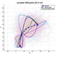
From above observations, we found out that it can be used to model distribution of trajectories that follow some prefixed locations. For example, let's assume that our problem is to find some paths that connect start and goal location while avoid obstacles. Then we the start and goal locations correspond to training data that the resulting path to follow at time '$t=0$' and '$t=t_T$' where '$t_T$' is the terminating time. As the GP posterior distributions is defined over all paths that follow given locations, we can easily sample paths from the distribution and select the path that does not overlap obstacles.
Figure below is the 500 sampled path given start and goal locations. It only took 27 ms to sample 500 paths.

'Enginius > Robotics' 카테고리의 다른 글
| Gaussian process path (0) | 2015.01.21 |
|---|---|
| Survey on people tracking for mobile robots (0) | 2015.01.19 |
| RSS 2014 papers (0) | 2014.12.12 |
| [ROS] ROS의 구조와 패키지 만드는 방법 (0) | 2014.08.21 |
| Installing ROS (0) | 2014.08.04 |