The Zernike polynomials were first proposed in 1934 by Zernike [22]. Their moment formulation appears to be one of the most popular, outperforming the alternatives [19] (in terms of noise resilience, information redundancy and reconstruction capability). The pseudo-Zernike formulation proposed by Bhatia and Wolf [3] further improved these characteristics. However, here we study the original formulation of these orthogonal invariant moments.
Complex Zernike moments [18] are constructed using a set of complex polynomials which form a complete orthogonal basis set defined on the unit disc ![]() . They are expressed as
. They are expressed as![]() Two dimensional Zernike moment:
Two dimensional Zernike moment:
![\begin{displaymath}
A_{mn} = \frac{m+1}{\pi} \int_{x} \int_{y} f(x,y)[V_{mn}(x,y)]^{*} ~dx~dy~~~~~\mbox{where $x^{2} + y^{2} \leq ~1$}
\end{displaymath}](http://homepages.inf.ed.ac.uk/rbf/CVonline/LOCAL_COPIES/SHUTLER3/img171.png)
and
where
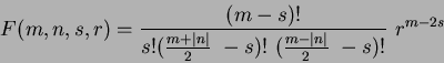
where:
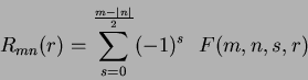
 | (53) |
| (54) | |||
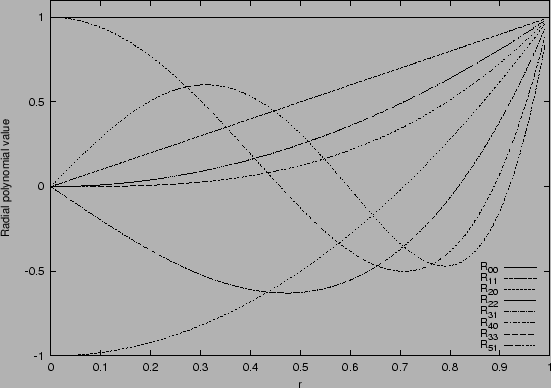
Figure 1.6 shows eight such radial responses, where it can been seen that the polynomials become more grouped, as they approach the edge of the unit disc (
![\begin{displaymath}
A_{mn} = \frac{m+1}{\pi} \sum_{x} \sum_{y} P_{xy}[V_{mn}(x,y)]^{*} ~~~~~\mbox{where $x^{2} + y^{2} \leq ~1$}
\end{displaymath}](http://homepages.inf.ed.ac.uk/rbf/CVonline/LOCAL_COPIES/SHUTLER3/img195.png) | (55) |
where
However,
and
Further, the absolute value of a Zernike moment is rotation invariant as reflected in the mapping of the image to the unit disc. The rotation of the shape around the unit disc is expressed as a phase change, if
Subsections
Next: A note on image Up: Orthogonal moments Previous: Legendre momentsJamie Shutler 2002-08-15
'Enginius > Machine Learning' 카테고리의 다른 글
| ANN로 headPoseEstimate하기 (0) | 2012.06.05 |
|---|---|
| Markov Chain Monte Carlo (MCMC) and Gibbs Sampling example(MATLAB) (0) | 2012.05.31 |
| 푸리에 변환과 라플라스 변환 (18) | 2012.05.01 |
| Hierarchical Temporal Memory Prototype ver1.0.0 (4) | 2012.04.26 |
| 기계 학습과 수학적 뒷받침 (0) | 2012.04.26 |


