What?
The code provided here originally demonstrated the main algorithms from Rasmussen and Williams: Gaussian Processes for Machine Learning. It has since grown to allow more likelihood functions, further inference methods and a flexible framework for specifying GPs. It does not currently contain inference methods for sparse approximations. Other GP packages can be found here.
The code is written by Carl Edward Rasmussen and Hannes Nickisch; it runs on both Octave 3.2.x and Matlab® 7.x. The code is based on previous versions written by Carl Edward Rasmussen and Chris Williams.
Download, Install and Documentation
All the code including demonstrations and html documentation can be downloaded in a tar or zip archive file.
Minor changes and incremental bugfixes are documented in the changelog. Please read the copyright notice.
After unpacking the tar or zip file you will find 6 subdirectories: cov, doc, inf, lik, mean and util. It is not necessary to install anything to get started, just run the startup.m script to set your path.
Details about the directory contents and on how to compile mex files can be found in the README. The getting started guide is the remainder of the html file you are currently reading (also available at http://gaussianprocess.org/gpml/code/matlab/doc). A Developer's Guide containing technical documentation is found in manual.pdf, but for the casual user, the guide is below.
Theory
Gaussian Processes (GPs) can conveniently be used for Bayesian supervised learning, such as regression and classification. In its simplest form, GP inference can be implemented in a few lines of code. However, in practice, things typically get a little more complicated: you might want to use complicated covariance functions and mean functions, learn good values for hyperparameters, use non-Gaussian likelihood functions (rendering exact inference intractable), use approximate inference algorithms, or combinations of many or all of the above. This is what the GPML software package does.
Gaussian Process는 regression과 classification과 같은 Bayesian supervised learning에 쉽게 사용될 수 있다. 가장 간단하게 구현한다면 GP는 단 몇 줄 만으로도 구현이 가능하다. 하지만 실제로 사용할 때는 더 복잡한 것들이 필요할 때가 있다. 더 복잡한 구조의 covariance function이나 mean function을 사용해서 hyper-parameter를 구해야할 때도 있고, non-Gaussian likelihood function을 사용해야할 때도 있고, approximate inference algorithmms이나 이들의 combination을 사용해야할 때도 있기 때문이다. 이것이 GPML software package가 필요한 이유이다.
Before going straight to the examples, just a brief note about the organization of the package. There are four types of objects which you need to know about:
예제로 바로 넘어가기 전에 이 package의 구조에 대해서 간단히 설명하겠다. 여기에는 너가 알아야할 네 가지 object가 있다.
- Gaussian Process
- A Gaussian Process is fully specified by a mean function and a covariance function. These functions are specified separately, and consist of a specification of a functional form as well as a set of parameters called hyperparameters, see below.
Gaussian Process는 mean function과 covariance function으로 모두 설명 가능하다. 이들 함수는 hyperparameter라는 변수를 갖는 함수이다.
- Mean functions
- Several mean functions are available, all start with the four letters mean and reside in the mean directory. An overview is provided by the meanFunctions help function (type help meanFunctions to get help), and an example is the meanLinearfunction.
- 여러 종류의 mean function이 사용가능하다. 이들은 모두 mean이라는 네 글자로 시작되고, mean 폴더 내에 모여있다. overview는 meanFunctions help에 있고, 예제는 meanLinearfunction이다.
- Covariance functions
- There are many covariance functions available, all start with the three letters cov and reside in the cov directory. An overview is provided by the covFunctions help function (type help covFunctions to get help), and an example is thecovSEard "Squared Exponential with Automatic Relevance Determination" covariance function.
- 여러 종류의 covariance function이 사용 가능하고, 이들은 모두 cov라는 세 글자로 시작되며 cov 폴더 내에 존재한다. overview는 covFunctions help로 제공되고, 예제는 thecovSEard에 있다.
- mean function과 covariance function 둘 다, 두 가지 type이 있다: simple과 composite. simple type은 function의 이름으로 specify되고, composite function은 cell array를 이용해서 여러 component들을 합친다. Composite function들은 다른 composite function들로 이뤄지며, 매우 flexible하고 흥미로운 구조를 가능하게 한다. 예제들은 usageMean과 usuageCov함수에 있다.
- Hyperparameters
- GPs are typically specified using mean and covariance functions which have free parameters called hyperparameters. Also likelihood functions may have such parameters. These are encoded in a struct with the fields mean, cov and lik (some of which may be empty). When specifying hyperparameters, it is important that the number of elements in each of these struct fields, precisely match the number of parameters expected by the mean function, the covariance function and the likelihood functions respectively (otherwise an error will result). Hyperparameters whose natural domain is positive are represented by their logarithms.
- GP는 일반적으로 hyperparameter를 갖는 mean function과 covariance function로 specify된다. 또한 likelihood 역시 이러한 parameter를 이용해서 표현된다. 이들 hyperparameter는 mean, cov, lik 구조체 안에 들어가있다. hyperparameter를 specify할 때, 이들 각 구초제 안에 있는 element의 수가 각각 mean, cov, lik 함수 안에 있는 parameter의 수와 정확히 맞추는 것이 중요하다. 0보다 큰 domain에 있는 parameter는 log가 취해져서 나타난다.
- Likelihood Functions
- The likelihood function specifies the probability of the observations given the latent function, i.e. the GP (and the hyperparameters). All likelihood functions begin with the three letters lik and reside in the lik directory. An overview is provided by the likFunctions help function (type help likFunctions to get help). Some examples are likGauss the Gaussian likelihood andlikLogistic the logistic function used in classification (a.k.a. logistic regression).
- likelihood function은 latent function이 주어졌을 때 observation의 확률을 나타낸다. likelihood function들은 lik 세 글자로 시작하며 lik 폴더 내에 있다. overview는 likFunctions help로 제공된다. likGauss, likLogistcs은 classification을 위해 제공된다.
- Inference Methods
- The inference methods specify how to compute with the model, i.e. how to infer the (approximate) posterior process, how to find hyperparameters, evaluate the log marginal likelihood and how to make predictions. Inference methods all begin with the three letters inf and reside in the inf directory. An overview is provided by the infMethods help file (type help infMethods to get help). Some examples are infExact for exact inference or infEP for the Expectation Propagation algorithm. Further usage examples are provided for both regression and classification. However, not all combinations of likelihood function and inference method are possible (e.g. you cannot do exact inference with a Laplace likelihood). An exhaustive compatibility matrix between likelihoods (rows) and inference methods (columns) is given in the table below:
- Inference model은 model을 어떻게 연산하는지 나타낸다. 예를 들어 posterior process를 어떻게 infer하고, hyperparameter를 어떻게 찾고, log marginal likelihood를 어떻게 계산하고, prediction을 어떻게 하는지. Inference method는 inf 세 글자로 시작하며 inf 폴더 내에 있다. -중략- likelihood와 inference의 compatibility에 대해선 아래 표를 봐라.
| Likelihood \ Inference | GPML name | Exact infExact | FITC infFITC | EP infEP | Laplace infLaplace | Variational Bayes infVB | LOO infLOO | type, output domain | alternate names |
| Gaussian | likGauss | regression, IR | |||||||
| Sech-squared | likSech2 | regression, IR | |||||||
| Laplacian | likLaplace | regression, IR | double exponential | ||||||
| Student's t | likT | regression, IR | |||||||
| Error function | likErf | classification, ±1 | probit regression | ||||||
| Logistic function | likLogistic | classification, ±1 | logistic regression logit regression |
All of the objects described above are written in a modular way, so you can add functionality if you feel constrained despite the considerable flexibility provided. Details about how to do this are provided in the developer documentation.
Practice
Using the GPML package is simple. There is only one single function to call: gp, it does posterior inference, learns hyperparameters, computes the marginal likelihood and makes predictions. Generally, the gp function takes the following arguments: a hyperparameter struct, an inference method, a mean function, a covariance function, a likelihood function, training inputs, training targets, and possibly test cases. The exact computations done by the function is controlled by the number of input and output arguments in the call. Here is part of the help message for the gp function (follow the link to see the whole thing):
GPML package를 사용하는 것은 간단하다. gp라고 불리는 단 하나의 함수 밖에 없다. 이 함수는 posterior inference, hyperparameter얻기, marginal likelihood 계산, prediction을 모두 수행한다. 일반적으로 gp는 다음의 argument를 인자로 받아드린다: hyperparameter 구조체, inference method, mean function, covariance function, likelihood function, training inputs, training targets, 그리고 test cases. exact computation은 input과 output argument의 수에 따라 정해진다. -후략-
function [varargout] = gp(hyp, inf, mean, cov, lik, x, y, xs, ys) [ ... snip ...] Two modes are possible: training or prediction: if no test cases are supplied, then the negative log marginal likelihood and its partial derivatives wrt the hyperparameters is computed; this mode is used to fit the hyperparameters. If test cases are given, then the test set predictive probabilities are returned. Usage:
두 가지 모델이 가능하다, 하나는 training이고 다른 하나는 prediction이다. 만약 test case가 없다면 negative log marginal
likelihood와 이것의 partial derivatives가 계산된다: 이 mode는 hyperparameter를 fit하는데 사용된다. 만약 test case가 주어
진다면 test set predictive probabilities가 반환된다.
training: [nlZ dnlZ ] = gp(hyp, inf, mean, cov, lik, x, y); prediction: [ymu ys2 fmu fs2 ] = gp(hyp, inf, mean, cov, lik, x, y, xs); or: [ymu ys2 fmu fs2 lp ] = gp(hyp, inf, mean, cov, lik, x, y, xs, ys);
[ .. snip ...]
Here x and y are training inputs and outputs, and xs and ys are test set inputs and outputs, nlZ is the negative log marginal likelihood and dnlZ its partial derivatives wrt the hyperparameters (which are used for training the hyperparameters). The prediction outputs areymu and ys2 for test output mean and covariance, and fmu and fs2 are the equivalent quenteties for the corresponding latent variables. Finally, lp are the test output log probabilities.
여기서 x와 y는 training input과 output이고, xs와 ys는 test set input과 output이다. nIZ는 negative log marginal likelihood이고, dnIZ는 hyperparameter로 구해진 partial derivatives이다. prediction output 중 ymu는 test output mean이고, ys2는 test output covariance이다. fmu와 fs2는 해당하는 latent variable에 대한 mu와 cov이다. 마지막으로 lp는 test output log probabilities이다.
Instead of exhaustively explaining all the possibilities, we will give two illustrative examples to give you the idea; one for regression and one for classification. You can either follow the example here on this page, or using the two scripts demoRegression anddemoClassification (using the scripts, you still need to follow the explanation on this page).
모든 가능성에 대해서 다 설명하기 보다, 우리는 두 개의 예제를 보여줄것이다. 하나는 regression이고, 다른 하나는 classification이다. 당신은 이 page에 있는 예제를 따를 수도 있고, 두 개의 script를 참고할 수도 있다.
Regression
You can either follow the example here on this page, or use the script demoRegression.
넌 이 페이지에 있는 예제를 따르거나, demoRegression script를 볼 수 있다.
This is a simple example, where we first generate n=20 data points from a GP, where the inputs are scalar (so that it is easy to plot what is going on). We then use various other GPs to make inferences about the underlying function.
이것은 간단한 예제이다. 우리는 20개의 data point를 GP로 부터 만든다. input은 scalar이다. 그리고 우리는 여러 다른 GP를 이용해서 underlying function에 대한 inference를 수행한다.
First, generate some data from a Gaussian process (it is not essential to understand the details of this):
먼저 gp에 사용될 data들을 만들자.
  clear all, close all

  meanfunc = {@meanSum, {@meanLinear, @meanConst}}; hyp.mean = [0.5; 1];
  covfunc = {@covMaterniso, 3}; ell = 1/4; sf = 1; hyp.cov = log([ell; sf]);
  likfunc = @likGauss; sn = 0.1; hyp.lik = log(sn);

  n = 20;
  x = gpml_randn(0.3, n, 1);
  K = feval(covfunc{:}, hyp.cov, x);
  mu = feval(meanfunc{:}, hyp.mean, x);
  y = chol(K)'*gpml_randn(0.15, n, 1) + mu + exp(hyp.lik)*gpml_randn(0.2, n, 1);

  plot(x, y, '+')
Above, we first specify the mean function meanfunc, covariance function covfunc of a GP and a likelihood function, likfunc. The corresponding hyperparameters are specified in the hyp structure:
The mean function is composite, adding (using meanSum function) a linear (meanLinear) and a constant (meanConst) to get an affine function. Note, how the different components are composed using cell arrays. The hyperparameters for the mean are given in hyp.mean and consists of a single (because the input will one dimensional, i.e. D=1) slope (set to 0.5) and an off-set (set to 1).
The number and the order of these hyperparameters conform to the mean function specification. You can find out how many hyperparameters a mean (or covariance or likelihood function) expects by calling it without arguments, such as feval(@meanfunc{:}). For more information on mean functions see meanFunctions and the directory mean/.
위에서, 우리는 먼저 mean function인 meanfunc, covariance function인 covfunc, 그리고 likelihood function인 likfunc를 specify한다. 이들에 해당하는 hyperparameter는 hyp 구조체에 명시되어있다.
mean functino은 composite하다. 즉, adding (using meanSum function) a linear (meanLinear) and a constant (meanConst) to get an affine function. 주의할 점은 어떻게 다른 component들이 cell array를 이용해서 compose되는지이다.
The covariance function is of the Matérn form with isotropic distance measure covMaterniso. This covariance function is also composite, as it takes a constant (related to the smoothness of the GP), which in this case is set to 3. The covariance function takes two hyperparameters, a characteristic length-scale ell and the standard deviation of the signal sf. Note, that these positive parameters are represented in hyp.cov using their logarithms. For more information on covariance functions see covFunctions andcov/.
covariance function은 Matern form이다. covariance function은 두 개의 hyperparameter를 갖는다. 여기서 주의할 점은 양의 값을 갖는 parameter는 log를 취해서 hyp.cov로 표현된다. 더 자세한 사항은 covFunctions와 cov폴더를 참조.
Finally, the likelihood function is specified to be Gaussian. The standard deviation of the noise sn is set to 0.1. Again, the representation in the hyp.lik is given in terms of its logarithm. For more information about likelihood functions, see likFunctions andlik/.
마지막으로 likelihood function은 Gaussian으로 정해졌다. 노이즈의 stdev는 0.1로 취해진다. 이 역시 log가 취해져서 정해진다. 더 자세한 사항은 likFunctions와 lik 폴더를 참조.
Then, we generate a dataset with n=20 examples. The inputs x are drawn from a unit Gaussian (using the gpml_randn utility, which generates unit Gaussian pseudo random numbers with a specified seed). We then evaluate the covariance matrix K and the mean vector m by calling the corresponding functions with the hyperparameters and the input locations x. Finally, the targets y are computed by drawing randomly from a Gaussian with the desired covariance and mean and adding Gaussian noise with standard deviation exp(hyp.lik). The above code is a bit special because we explicitly call the mean and covariance functions (in order to generate samples from a GP); ordinarily, we would only directly call the gp function.
그리고 나서, 우리는 20개의 dataset를 만든다. input x는 unit Guassian으로 부터 만들어진다. 그리고 나서 우리는 covariance matrix K와 mean vector m을 주어진hyperparameter와 input x와 함께 구한다. 마지막으로, target y는 주어진 covariance와 mean과 noise로 정의된 Gaussian으로 부터 랜덤하게 그려진다. 위의 code는 약간 일반적이지 않는데 왜냐하면 우리가 mean과 cov함수를 직접 불렀기 때문이다; 일반적으로 우리는 gp함수를 직접 부른다.
Let's ask the model to compute the (joint) negative log probability (density) nlml (also called marginal likelihood or evidence) and to generalize from the training data to other (test) inputs z:
이렇게 주어진 dataset의 negative log probability와 marginal likelihood(nlml)를 계산하고 다른 test input z를 고려하자.
  nlml = gp(hyp, @infExact, meanfunc, covfunc, likfunc, x, y)

  z = linspace(-1.9, 1.9, 101)';
  [m s2] = gp(hyp, @infExact, meanfunc, covfunc, likfunc, x, y, z);

  f = [m+2*sqrt(s2); flipdim(m-2*sqrt(s2),1)];
  fill([z; flipdim(z,1)], f, [7 7 7]/8)
  hold on; plot(z, m); plot(x, y, '+')
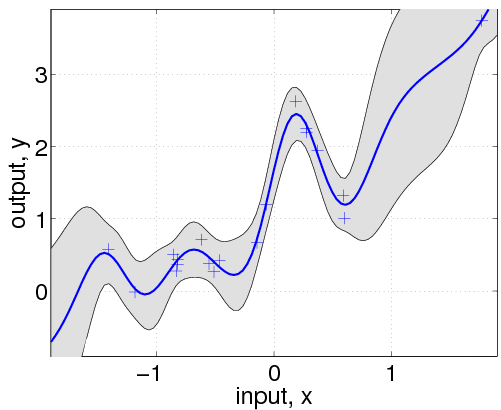
The gp function is called with a struct of hyperparameters hyp, and inference method, in this case @infExact for exact inference and the mean, covariance and likelihood functions, as well as the inputs and outputs of the training data. With no test inputs, gp returns the negative log probability of the training data, in this example nlml=11.97.
gp 함수는 hyp hyperparameter 구조체와 @infExact inference method와 주어진 mean, covariance, likelihood, input x, output y와 함께 불린다. test input이 없으면 gp는 training data의 negative log probability를 return하고, 이 경우 nlml은 11.97이다.
To compute the predictions at test locations we add the test inputs z as a final argument, and gp returns the mean m variance s2 at the test location. The program is using algorithm 2.1 from the GPML book. Plotting the mean function plus/minus two standard deviations (corresponding to a 95% confidence interval):
test location에서 prediction을 계산하기 위해선, 우리는 test input z를 마지막 argument로 넣어주구, gp는 각 test location에서 평균 m과 variance s2를 반환한다. 이 프로그램은 GPML 책의 알고리즘 2.1을 사용한다. 그래프 그리는 것은 mean값에 2 stdev 만큼 plus/minus한 값으로 그린다.
Typically, we would not a priori know the values of the hyperparameters hyp, let alone the form of the mean, covariance or likelihood functions. So, let's pretend we didn't know any of this. We assume a particular structure and learn suitable hyperparameters:
일반적으로 우리는 hyp hyperparameter에 대해서 알지 못한다. 그래서 우리가 이들 mean, covariance, likelihood를 모른다고 가정하자. 우리는 특정 구조를 가정하고, 가능한 hyperparameter를 학습하자.
covfunc = @covSEiso; hyp2.cov = [0; 0]; hyp2.lik = log(0.1);
First, we guess that a squared exponential covariance function covSEiso may be suitable. This covariance function takes two hyperparameters: a characteristic length-scale and a signal standard deviation (magnitude). These hyperparameters are non-negative and represented by their logarithms; thus, initializing hyp2.cov to zero, correspond to unit characteristic length-scale and unit signal standard deviation. The likelihood hyperparameter in hyp2.lik is also initialized. We assume that the mean function is zero, so we simply ignore it (and when in the following we call gp, we give an empty argument for the mean function).
먼저, 우리는 squared exponential covariance function covSEiso가 적합할 것이라고 가정한다. 이 covariance function은 두 개의 hyperparameter를 갖는다; characteristic length-scale과 signal standard deviation이다. 이들 hyperparameter들은 음수가 아니며, log가 취해져서 나타난다. hyp2.cov를 0으로 초기화하는 것은 각 parameter를 1로 하는 것과 같다. (log 1 = 0) 인 likelihood hyperparameter인 hyp2.lik 역시 초기화된다. 우리는 mean function은 0일 것이라고 가정하기 때문에 이는 무시한다.
  hyp2 = minimize(hyp2, @gp, -100, @infExact, [], covfunc, likfunc, x, y);
  exp(hyp2.lik)
  nlml2 = gp(hyp2, @infExact, [], covfunc, likfunc, x, y)

  [m s2] = gp(hyp2, @infExact, [], covfunc, likfunc, x, y, z);
  f = [m+2*sqrt(s2); flipdim(m-2*sqrt(s2),1)];
  fill([z; flipdim(z,1)], f, [7 7 7]/8)
  hold on; plot(z, m); plot(x, y, '+')
In the following line, we optimize over the hyperparameters, by minimizing the negative log marginal likelihood w.r.t. the hyperparameters. The third parameter in the call to minimize limits the number of function evaluations to a maximum of 100. The inferred noise standard deviation is exp(hyp2.lik)=0.15, somewhat larger than the one used to generate the data (0.1). The final negative log marginal likelihood is nlml2=14.13, showing that the joint probability (density) of the training data is about exp(14.13-11.97)=8.7 times smaller than for the setup actually generating the data. Finally, we plot the predictive distribution.
다음 line에서 우리는 negative log marginal likelihood를 이용해서 hyperparameter를 최적화한다. minimize의 세 번째 parameter는 evaluation을 하는 한계를 100으로 정해준다. inferred noise standard deviatioin은 exp(hyp2.kil) = 0.15이고, 우리가 이전에 주었던 0.1보다는 크다. 마지막 negative log marginal likelihood는 nlml2 = 14.13이고, 이는 training data의 joint probability density가 data를 만들 때 setup했던 것보다 8.7배 더 작다는 것을 나타낸다. 마지막으로 우리는 predictive distribution을 plot한다.
This plot shows clearly, that the model is indeed quite different from the generating process. This is due to the different specifications of both the mean and covariance functions. Below we'll try to do a better job, by allowing more flexibility in the specification.
이번 plot은 분명히 보여주는데, model이 generation process와는 상당히 다르다는 것을 보여준다. 이것은 mean과 covariance 모두 다른 값을 넣어주었기 때문이다. 아래 우리는 specification에 flexibility를 줌으로 더 좋은 결과를 얻으려고 할 것이다.
Note that the confidence interval in this plot is the confidence for the distribution of the (noisy) data. If instead you want the confidence region for the underlying function, you should use the 3rd and 4th output arguments from gp as these refer to the latent process, rather than the data points.
여기서 주의할 것은 이번 plot에서 confidence interval은 noise가 섞인 data의 distribution의 confidence이다. 만약 너가 underlying function에 대한 confidence region을 원한다면, 너는 gp의 data point 대신에 latent process를 위한 세 번째와 네 번째 output argument을 사용해야한다.
  hyp.cov = [0; 0]; hyp.mean = [0; 0]; hyp.lik = log(0.1);
  hyp = minimize(hyp, @gp, -100, @infExact, meanfunc, covfunc, likfunc, x, y);
  [m s2] = gp(hyp, @infExact, meanfunc, covfunc, likfunc, x, y, z);

  f = [m+2*sqrt(s2); flipdim(m-2*sqrt(s2),1)];
  fill([z; flipdim(z,1)], f, [7 7 7]/8)
  hold on; plot(z, m); plot(x, y, '+');
Here, we have changed the specification by adding the affine mean function. All the hyperparameters are learnt by optimizing the marginal likelihood.
여기서, 우리는 affine mean function을 더함으로서 specification을 바꿨다(앞에선 mean을 쓰지 않았다). 모든 hyperparameter들은 marginal likelihood를 최적화함으로 학습한다.
This shows that a much better fit is achieved when allowing a mean function (although the covariance function is still different from that of the generating process).
이 결과는 mean function을 허용하면 더 좋은 결과가 나옴을 보여준다(covariance function은 generating process와는 여전히 다름에도)
Exercises for the reader
- Inference Methods
- Try using Expectation Propagation instead of exact inference in the above, by exchanging @infExact with @infEP. You get exactly identical results, why?
- Mean or Covariance
- Try training a GP where the affine part of the function is captured by the covariance function instead of the mean function. That is, use a GP with no explicit mean function, but further additive contributions to the covariance. How would you expect the marginal likelihood to compare to the previous case?
Large scale regression
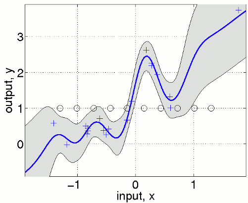
In case the number of training inputs x exceeds a few thousands, exact inference using infExact.m takes too long. We offer the FITC approximation based on a low-rank plus diagonal approximation to the exact covariance to deal with these cases. The general idea is to use inducing points u and to base the computations on cross-covariances between training, test and inducing points only.
만약 training input x가 수천을 넘는다면, infExact.m을 이용한 exact inference는 너무 오래 걸린다. 우리느 FITC approximation based on a low-rank plus diagonal approximation을 추천한다. general idea는 including point u를 사용하고, to base the computations on cross-covariance between training, test and including points only.
Ushe FITC approximation is very simple, we just have to wrap the covariance function covfunc into covFITC.m and call gp.m with the inference method infFITC.m as demonstrated by the following lines of code.
FITC approximation은 매우 간단한데, 우리는 covfunc를 conFITC.m으로 싸면되고, gp.m을 infFITC.m inference method로 부른다. (아래 설명 - )
nu = fix(n/2); u = linspace(-1.3,1.3,nu)';
covfuncF = {@covFITC, {covfunc}, u};
[mF s2F] = gp(hyp, @infFITC, meanfunc, covfuncF, likfunc, x, y, z);
We define equispaced inducing points u that are shown in the figure as black circles. Note that the predictive variance is overestimated outside the support of the inducing inputs. In a multivariate example where densely sampled inducing inputs are infeasible, one can simply use a random subset of the training points.
우리는 동일 간격을 갖는 point u를 정의하고, 이는 그림에서 검은 원으로 표시된다. 주의할 점은 predictive variance는 input 밖에서는 overestimate된다. multivariate example에서는 샘플링이 힘들기 때문에 training points의 subset에서 랜덤하게 뽑아서 사용한다.
nu = fix(n/2); iu = randperm(n); iu = iu(1:nu); u = x(iu,:);
Classification
You can either follow the example here on this page, or use the script demoClassification.
The difference between regression and classification isn't of fundamental nature. We can use a Gaussian process latent function in essentially the same way, it is just that the Gaussian likelihood function often used for regression is inappropriate for classification. And since exact inference is only possible for Gaussian likelihood, we also need an alternative, approximate, inference method.
regression과 classification의 차이는 자연의 법칙은 아니다. 우리는 Gaussian process latent function을 동일하게 사용할 수 있는데, 이렇게 되는 것은 다만 regression에 쓰이는 Gaussian likelihood function이 가끔 classification에 사용될 수 없기 때문이다. 그리고 exact inference는 Gaussian likelihood에서만 사용가능하므로, 우리는 또한 다른 대략적인 inference method가 필요하다.
Here, we will demonstrate binary classification, using two partially overlapping Gaussian sources of data in two dimensions. First we generate the data:
여기서 우리는 binary classification을 소개한다. 2차원에서 두 개의 겹치는 Gaussian sources를 이용한다. 먼저 우리는 data를 만든다.
  clear all, close all

  n1 = 80; n2 = 40;                   % number of data points from each class
  S1 = eye(2); S2 = [1 0.95; 0.95 1];           % the two covariance matrices
  m1 = [0.75; 0]; m2 = [-0.75; 0];                            % the two means

  x1 = bsxfun(@plus, chol(S1)'*gpml_randn(0.2, 2, n1), m1);
  x2 = bsxfun(@plus, chol(S2)'*gpml_randn(0.3, 2, n2), m2);

  x = [x1 x2]'; y = [-ones(1,n1) ones(1,n2)]';
  plot(x1(1,:), x1(2,:), 'b+'); hold on;
  plot(x2(1,:), x2(2,:), 'r+');
120 data points are generated from two Gaussians with different means and covariances. One Gaussian is isotropic and contains 2/3 of the data (blue), the other is highly correlated and contains 1/3 of the points (red). Note, that the labels for the targets are ±1 (andnot 0/1).
서로 다른 mean과 covariance를 갖는 두 개의 Gaussian으로 부터 120 point를 형성한다.
In the plot, we superimpose the data points with the posterior equi-probability contour lines for the probability of class two given complete information about the generating mechanism
plot에선, data point와 동일한-확률을 갖는 contour를 같이 그렸다.
  [t1 t2] = meshgrid(-4:0.1:4,-4:0.1:4);
  t = [t1(:) t2(:)]; n = length(t);                 % these are the test inputs
  tmm = bsxfun(@minus, t, m1');
  p1 = n1*exp(-sum(tmm*inv(S1).*tmm/2,2))/sqrt(det(S1));
  tmm = bsxfun(@minus, t, m2');
  p2 = n2*exp(-sum(tmm*inv(S2).*tmm/2,2))/sqrt(det(S2));
  contour(t1, t2, reshape(p2./(p1+p2), size(t1)), [0.1:0.1:0.9]);
We specify a Gaussian process model as follows: a constant mean function, with initial parameter set to 0, a squared exponential with automatic relevance determination (ARD) covariance function covSEard. This covariance function has one characteristic length-scale parameter for each dimension of the input space, and a signal magnitude parameter, for a total of 3 parameters (as the input dimension is D=2). ARD with separate length-scales for each input dimension is a very powerful tool to learn which inputs are important for predictions: if length-scales are short, inputs are very important, and when they grow very long (compared to the spread of the data), the corresponding inputs will be largely ignored. Both length-scales and the signal magnitude are initialized to 1 (and represented in the log space). Finally, the likelihood function likErf has the shape of the error-function (or cumulative Gaussian), which doesn't take any hyperparameters (so hyp.lik does not exist).
  meanfunc = @meanConst; hyp.mean = 0;
  covfunc = @covSEard; ell = 1.0; sf = 1.0; hyp.cov = log([ell ell sf]);
  likfunc = @likErf;

  hyp = minimize(hyp, @gp, -40, @infEP, meanfunc, covfunc, likfunc, x, y);
  [a b c d lp] = gp(hyp, @infEP, meanfunc, covfunc, likfunc, x, y, t, ones(n, 1));

  plot(x1(1,:), x1(2,:), 'b+'); hold on; plot(x2(1,:), x2(2,:), 'r+')
  contour(t1, t2, reshape(exp(lp), size(t1)), [0.1:0.1:0.9]);
We train the hyperparameters using minimize, to minimize the negative log marginal likelihood. We allow for 40 function evaluations, and specify that inference should be done with the Expectation Propagation (EP) inference method @infEP, and pass the usual parameters. Training is done using algorithm 3.5 and 5.2 from the gpml book. When computing test probabilities, we call gp with additional test inputs, and as the last argument a vector of targets for which the log probabilities lp should be computed. The fist four output arguments of the function are mean and variance for the targets and corresponding latent variables respectively. The test set predictions are computed using algorithm 3.6 from the gpml book. The contour plot for the predictive distribution is shown below. Note, that the predictive probability is fairly close to the probabilities of the generating process in regions of high data density. Note also, that as you move away from the data, the probability approaches 1/3, the overall class probability.
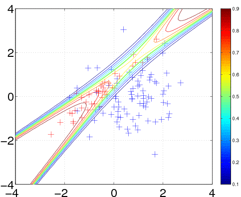
Examining the two ARD characteristic length-scale parameters after learning, you will find that they are fairly similar, reflecting the fact that for this data set, both inputs important.
Exercise for the reader
- Inference Methods
- Use the Laplace Approximation for inference @infLaplace, and compare the approximate marginal likelihood for the two methods. Which approximation is best?
- Covariance Function
- Try using the squared exponential with isotropic distance measure covSEiso instead of ARD distance measure covSEard. Which is best?
Acknowledgements
Innumerable colleagues have helped to improve this software. Some of these are: John Cunningham, Máté Lengyel, Joris Mooij, Iain Murray and Chris Williams. Especially Ed Snelson helped to improve the code and to include sparse approximations.
Last modified: February 15th 2011
'Enginius > Machine Learning' 카테고리의 다른 글
| Linear Programming (0) | 2012.07.03 |
|---|---|
| Gaussian Process 논문 정리 (0) | 2012.06.30 |
| Gaussian Process (4) | 2012.06.21 |
| [Deep Learning ]RBM trained with Contrastive Divergence (6) | 2012.06.15 |
| 내가 만든 LDA in Matlab (3) | 2012.06.10 |


